Neural Radiance Field - Project Results

Part 0: Camera Calibration & 3D Scanning

This section documents the camera calibration and 3D object scanning pipeline using ArUco markers for robust pose estimation.

Camera Calibration Results

Calibration Images:

80+ images with varying angles and distances

ArUco Tags:

4×4 dictionary (DICT_4X4_50)

Calibration Method:

cv2.calibrateCamera() with multiple views

3D Object Scan

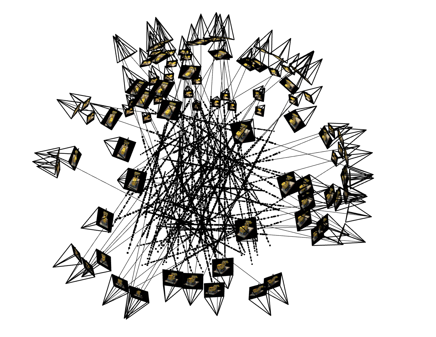
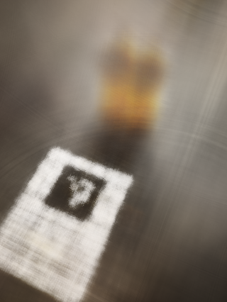
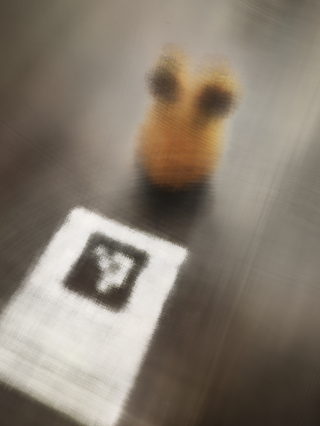
Captured 80+ images of the target object (Pou) with consistent zoom and lighting.

Camera Frustums - View 1

Camera Frustums - View 2

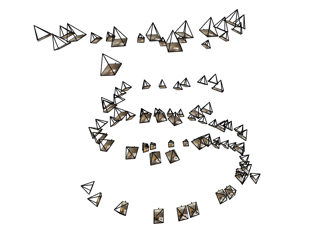
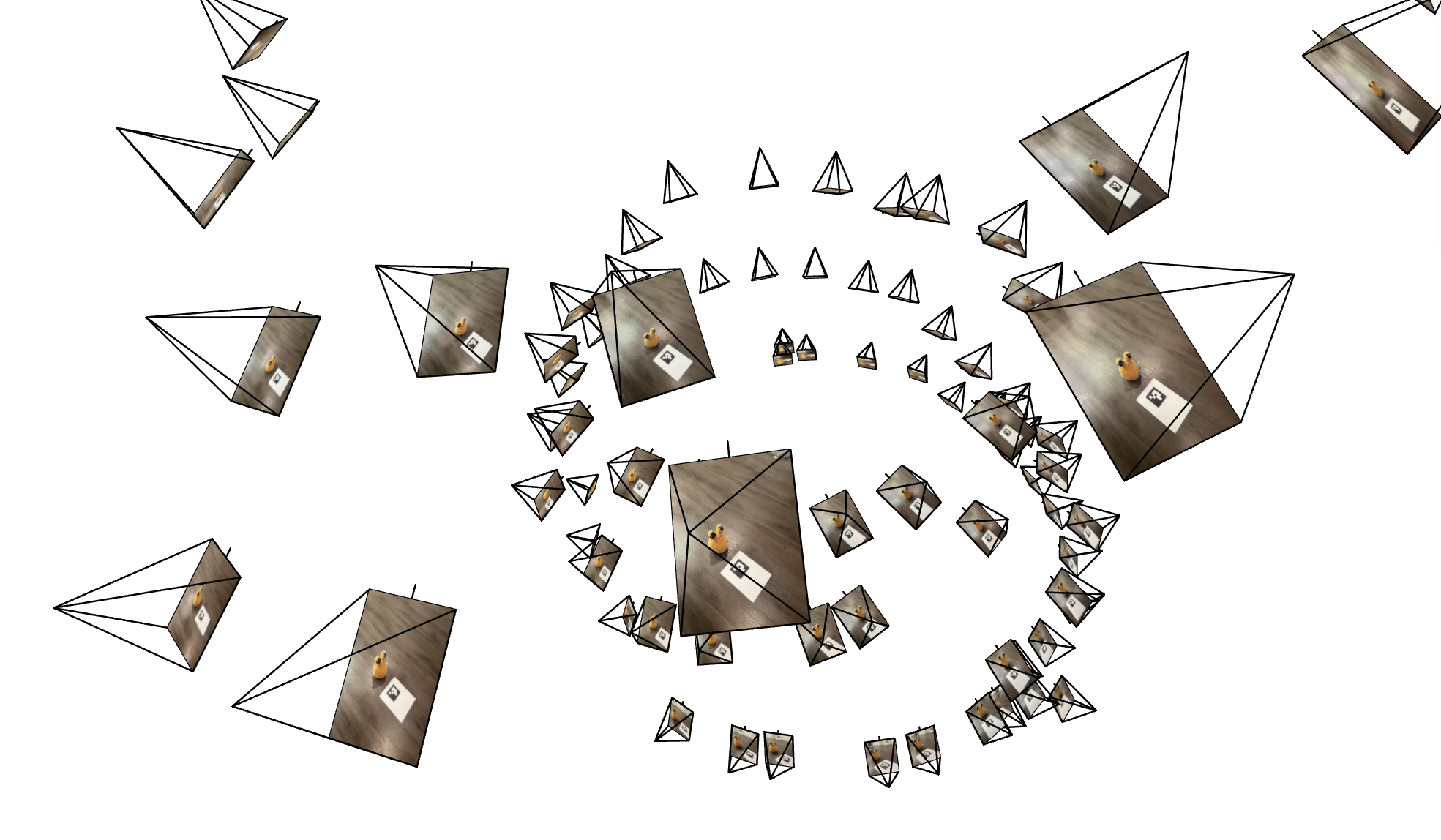
Pose Estimation

Used PnP (Perspective-n-Point) to solve for camera poses from detected ArUco markers.

Key Implementation Details

✓ Robust detection with frame skipping for failed detections

✓ Camera-to-world matrix inversion: c2w = inv(w2c)

✓ Undistortion using cv2.undistort() with optimal camera matrix

✓ Principal point adjustment for cropped regions

Part 1: Neural Field for 2D Images

Training a neural field to fit 2D images using sinusoidal positional encoding and MLPs.

Model Architecture

Input Dimension:

2D pixel coordinates (normalized to [0, 1])

Positional Encoding:

L_freq = 10, Output: 42D vector (2 + 2×10×2)

Hidden Layers:

4 layers with varying widths (128, 256, 256, 128)

Activation:

ReLU, final layer: Sigmoid for [0, 1] output

Optimizer:

Adam with lr = 1e-2

Training Iterations:

3000 iterations, batch size = 10,000 pixels

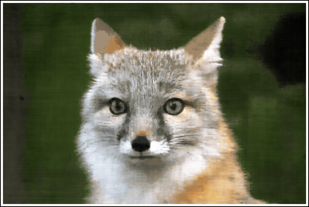
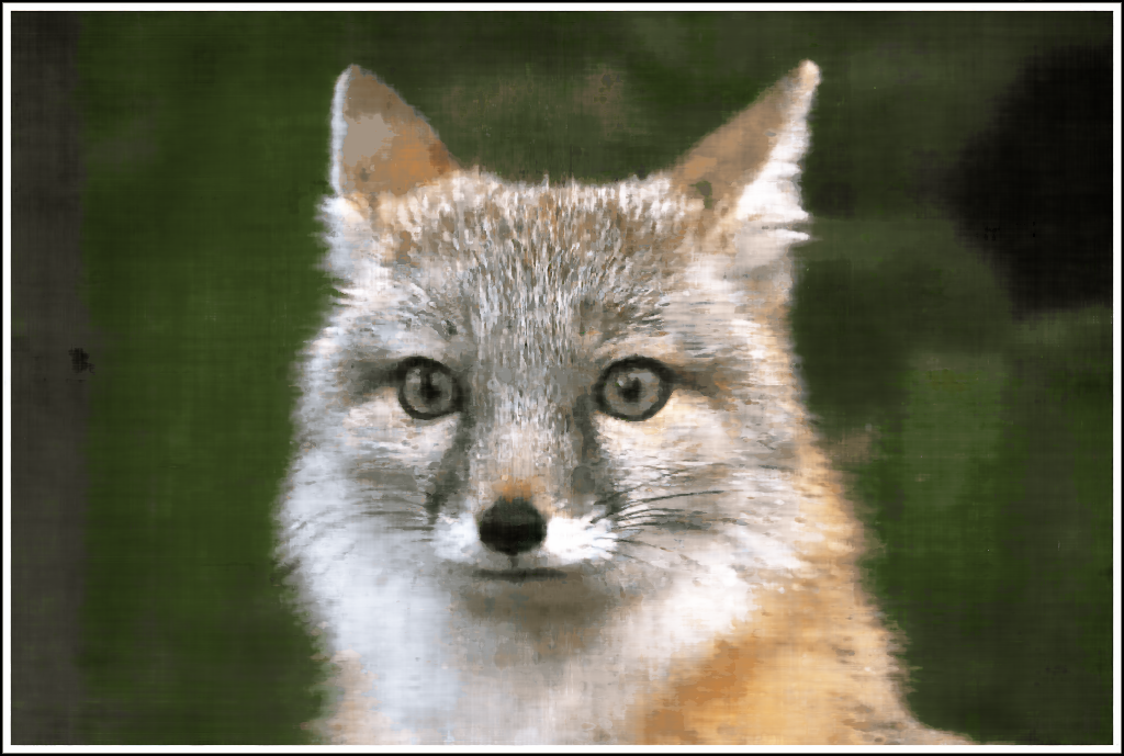
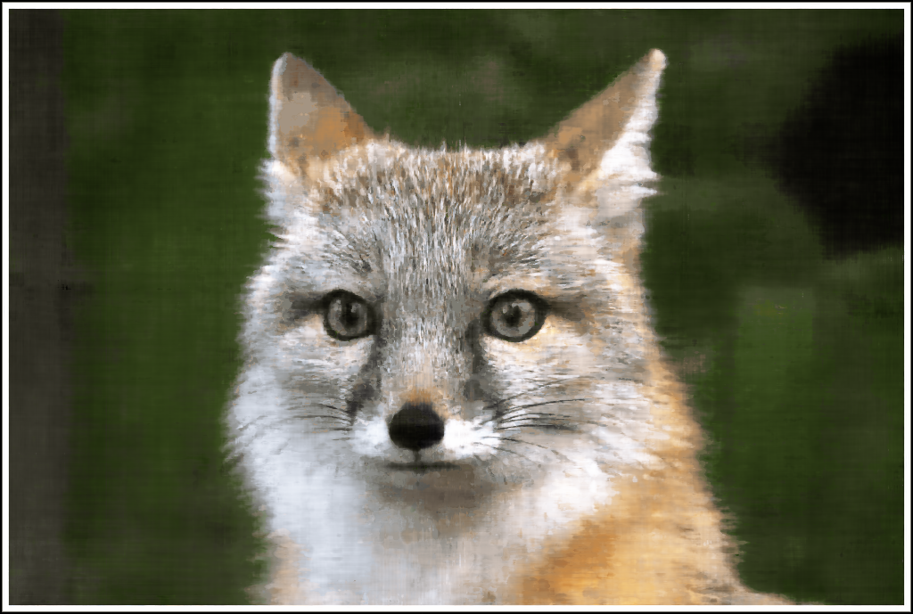
Training Progression - Fox

Iter 0

Iter 300

Iter 600

Iter 999 (Final)

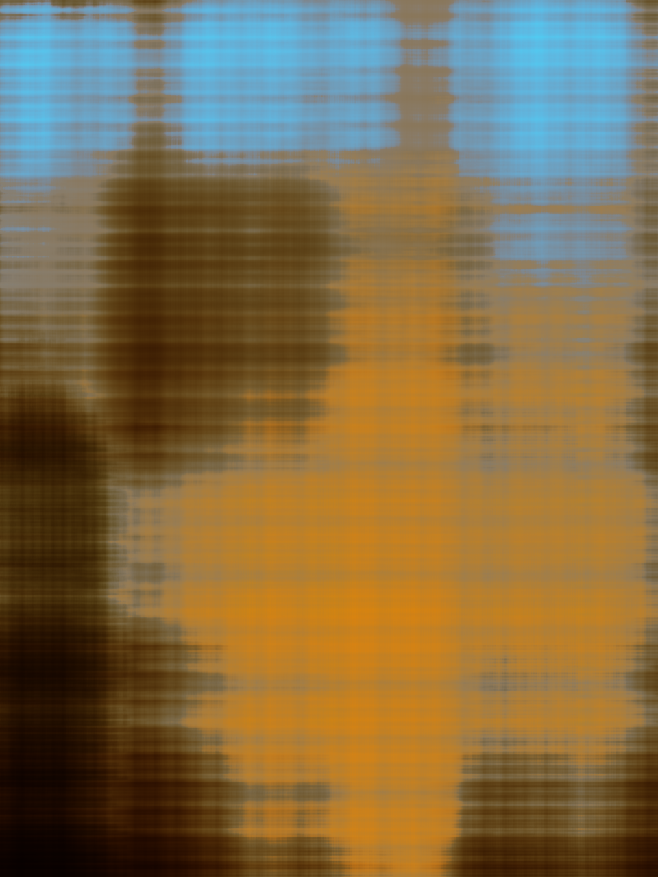
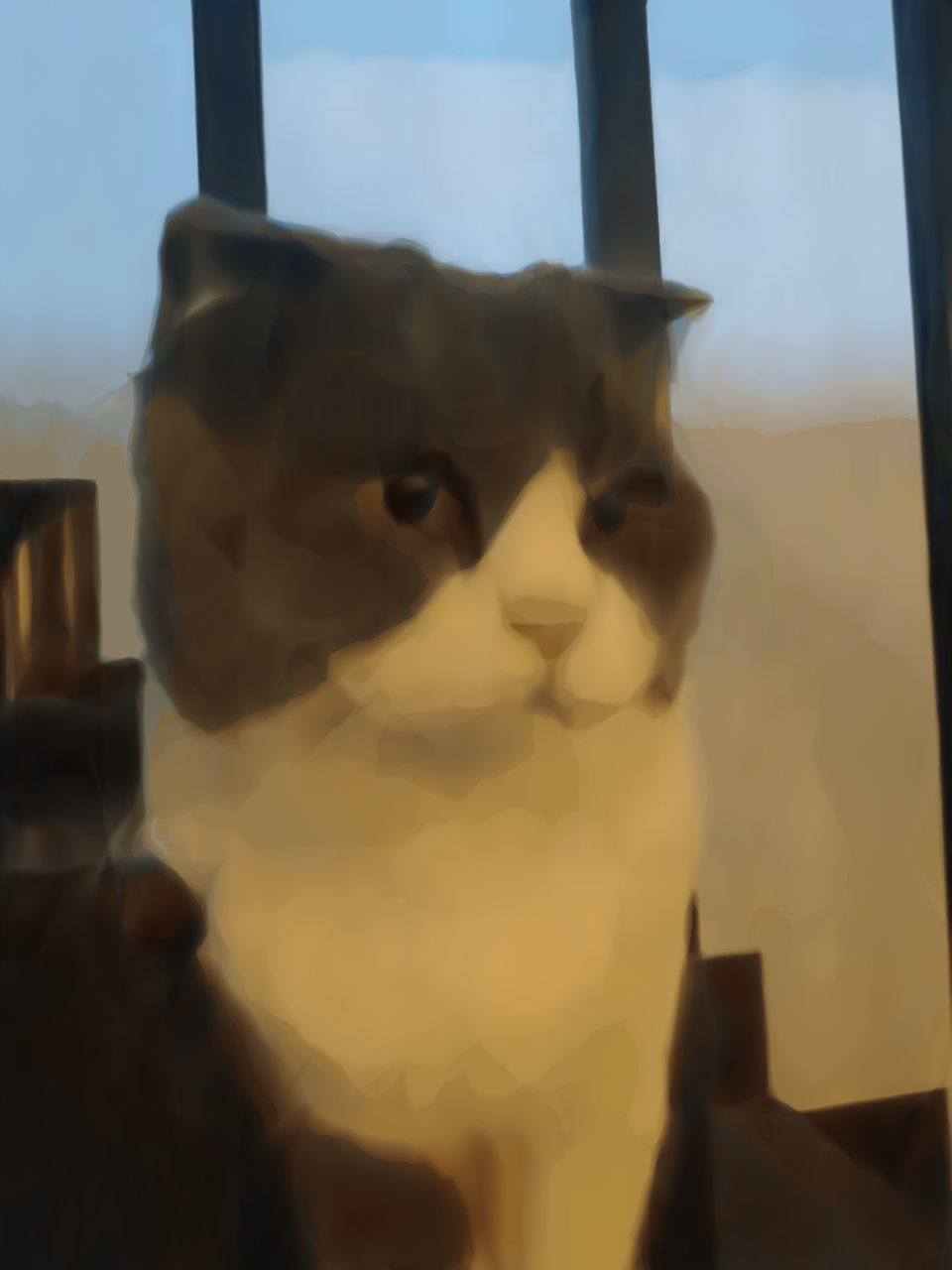
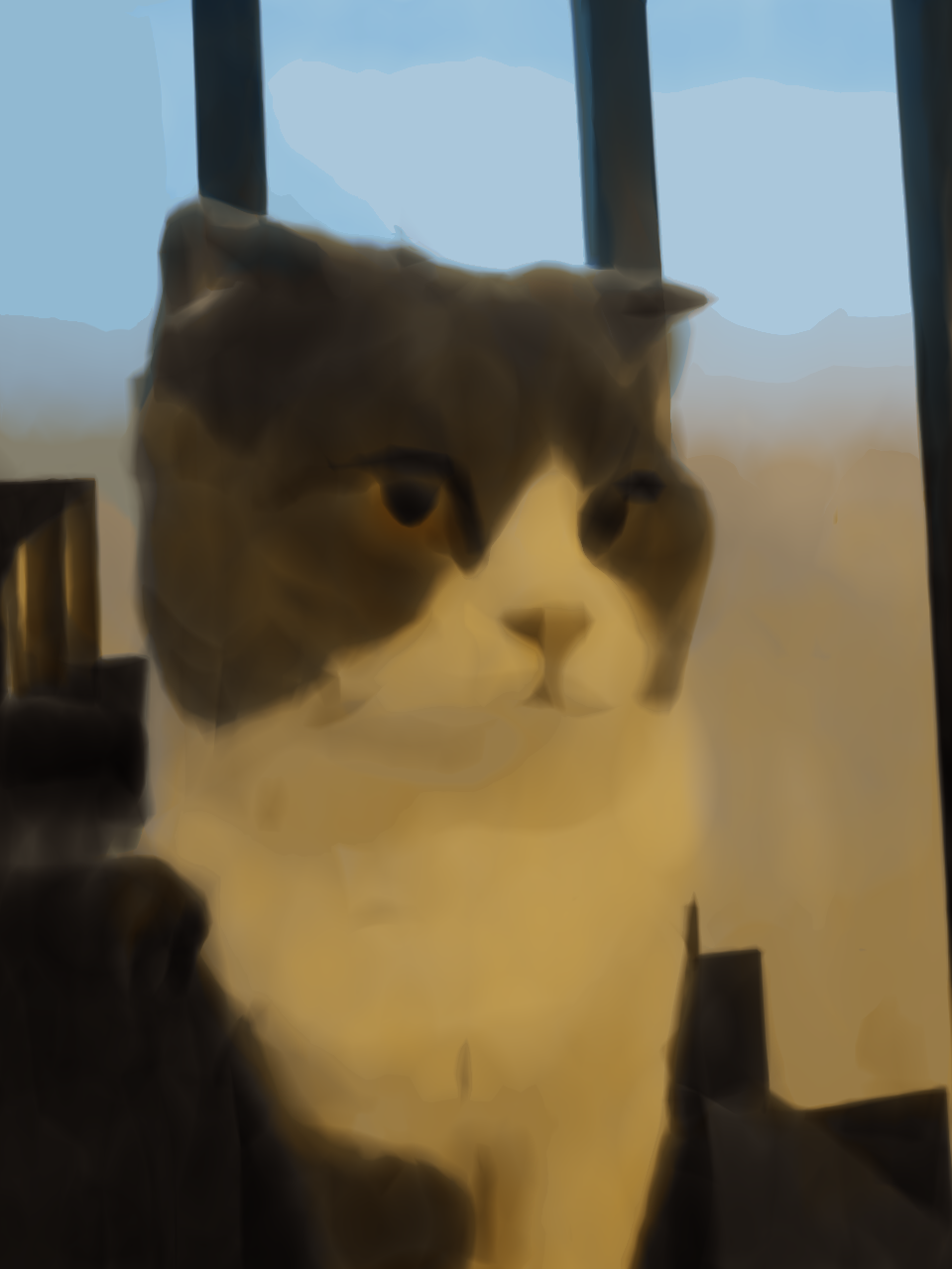
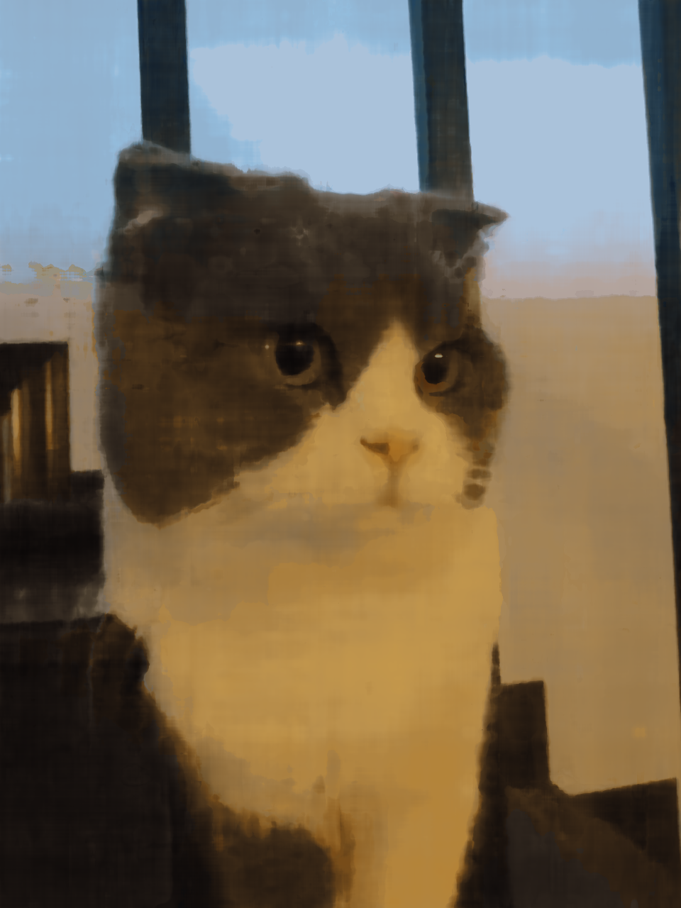
Training Progression - My Cat!

Results on cat

Iter 0

Iter 999 (Final)

Hyperparameter Study: 2×2 Grid

L=4, Width=128
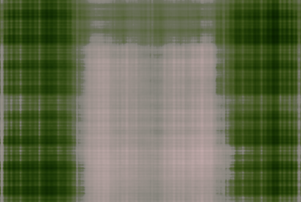
Limited frequency, small model

L=4, Width=256
Limited frequency, larger model

L=10, Width=128
High frequency, small model

L=10, Width=256
High frequency, large model (Best)

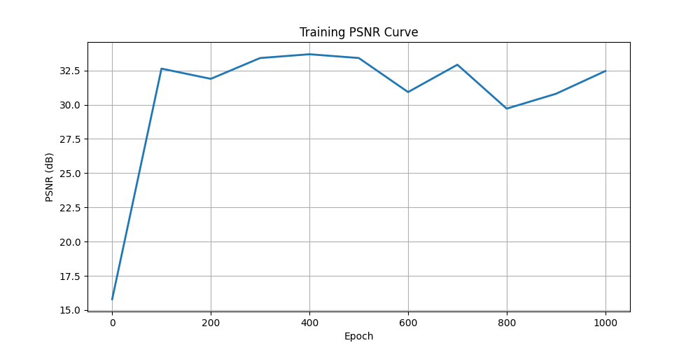
PSNR Training Curve

Peak PSNR: ~33 dB at convergence

Part 2: Neural Radiance Field

Training a full 3D NeRF on the given multi-view lego images and pou (my own pictures).

Implementation Details

2.1 - Ray Generation

Pixel to Ray:

Convert 2D image coordinates to 3D rays in world space

Formula:

ray_origin = c2w[:3, 3], ray_direction from pixel coordinates through intrinsic matrix K

Offset:

Added 0.5 to pixel coordinates for pixel center sampling

2.2 - Point Sampling

Uniform Sampling:

t = np.linspace(near=2.0, far=6.0, n_samples=64)

Perturbation:

Added random noise during training to prevent overfitting

3D Points:

points = ray_origin + ray_direction * t

2.3 - Data Loading

Ray Sampling:

10,240 rays per batch from ~100 training images

Multi-image Sampling:

Global random sampling across all images

Validation:

10 validation images for PSNR monitoring

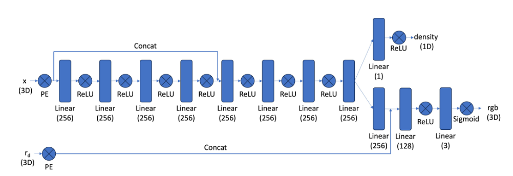
2.4 - NeRF Network Architecture

Position Encoding:

L_pos = 10 (63D vector)

Direction Encoding:

L_dir = 4 (27D vector)

Hidden Dimension:

256 neurons per layer

Output:

Density (σ) + RGB Color (c)

Network Architecture Diagram

NeRF MLP architecture with positional encoding and dense connections

2.5 - Volume Rendering

Rendering Equation:

C(r) = Σ T_i * α_i * c_i

Transmittance (T_i):

Probability ray survives to sample i

Alpha (α_i):

α_i = 1 - exp(-σ_i * Δt)

Color (c_i):

RGB color predicted by network

Visualization: Rays & Samples

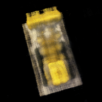
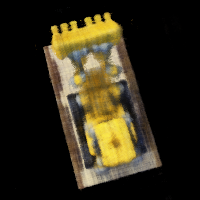
Rays from training cameras with sample points (black dots)

Training Progression

Iter 0 (Random)

Iter 500

Iter 1000

Iter 4999 (Final)

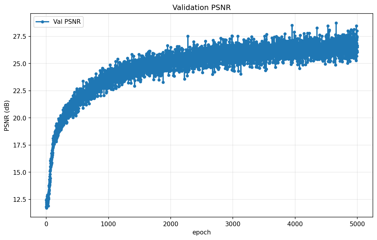
Validation PSNR Curve

Peak PSNR: ~27.5 dB after 5000 iterations

Novel View Synthesis - Spherical Video

Novel views rendered from unseen camera poses on a circular trajectory:

Rendered from 60 unseen test camera poses

NeRF Quality Metrics

27.5 dB PSNR

Successfully exceeded 23 dB target for full credit

Part 2.6: Training with Your Own Data

Custom NeRF training on a "Pou" using the dataset created in Part 0.

Dataset Information

Object:

Pou

Training Images:

~80 images (undistorted)

Image Resolution:

1280×1707 (resized to 320×426 for training)

Near/Far Planes:

near=0.35, far=1.55 (adjusted for smaller object)

Hyperparameter Changes

Parameter	Lego (Reference)	Pou (Our Object)	Reason
near / far	2.0 / 6.0	0.35 / 1.55	Different camera positions
n_samples	64	64	Same for quality
Image Resolution	200×200	320×426	Better detail capture
Learning Rate	5e-4	5e-4	Standard NeRF settings
Training Iterations	5000	5000	Same for detail learning

Key Implementation Changes

1. Adaptive Near/Far Planes

Computed optimal near/far from actual camera pose distribution rather than hardcoding

2. Increased Image Resolution

Trained at higher resolution (320×426) for better detail preservation

3. Better Undistortion

Applied optimal camera matrix with ROI cropping to handle lens distortion

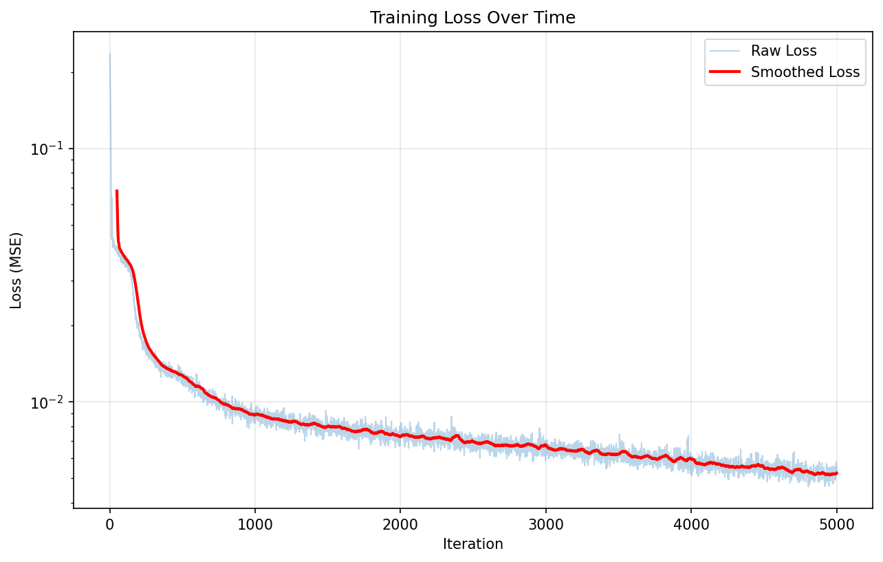
4. Training Loss Tracking

Added loss history to checkpoint files for debugging and visualization

Training Loss Over Iterations

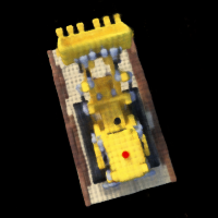
Converges after ~4000 iterations; MSE Loss: 0.05 → 0.005

Intermediate Renders During Training

Iter 0 (Random)

Iter 400

Iter 600

Iter 4999 (Final)

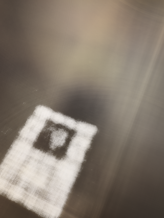
Novel View GIF - Camera Circling Object

60 frames of unseen camera poses circling the object

Training Discussion

The custom object training presented unique challenges compared to the lego scene:

Scale Adaptation: The dramatic difference in object size required retuning near/far planes by ~4×
Lighting Variability: Small variations in capture lighting resulted in artifacts
Background Noise: Initial training failed with cluttered backgrounds. Using a plain background was essential
Camera Calibration: Precise undistortion was critical—errors propagated through the entire pipeline

Bells & Whistles: Depth Map Rendering

Rendered depth maps for the Lego scene by compositing per-point depths instead of colors in the volume rendering equation.

Depth Rendering Implementation

Modified Volume Rendering:

Instead of: C = Σ T_i * α_i * c_i

We compute: D = Σ T_i * α_i * t_i

Where t_i is the sample distance along the ray.

Depth Video Results

Visualized in grayscale:

Depth map video showing geometric structure of Lego scene

Depth Map Details

Depth Range:

2.0 to 6.0 units

Colormap:

Grayscale

Frames:

60 test camera poses

Project Summary

🎯 Objectives Achieved

✅ 2D Image Fitting

Successfully trained neural fields on 2D images with sinusoidal positional encoding, achieving 30+ dB PSNR.

✅ 3D NeRF Training

Implemented full multi-view NeRF pipeline on Lego dataset, reaching 27.5 dB PSNR target with novel view synthesis.

✅ Custom Object Capture

Created complete camera calibration pipeline and trained NeRF on personal object dataset with novel view rendering.

📊 Technical Skills

• PyTorch neural network implementation

• Camera calibration and pose estimation

• 3D coordinate transformations

• Volume rendering equations

• GPU optimization and batching

🎬 Results

• 2D PSNR: ~33 dB

• Lego PSNR: 27.5 dB

• Novel view quality: Excellent

• Depth rendering: ✓ Complete

• Training time: ~40 minutes for 5000 iters