Flow Matching from Scratch

Overview

This project explores generative modeling through flow matching on MNIST. We start with a simple one-step denoiser, then progress to time-conditioned and class-conditioned UNets for iterative image generation. The core idea is to learn a velocity field that transforms noise into realistic images.

Key Concepts

Denoising: Training a network to remove noise from images
Flow Matching: Learning a velocity field from noisy to clean data
Time Conditioning: Injecting timestep information into the network
Class Conditioning: Controlling generation with class labels
Classifier-Free Guidance: Improving quality through guidance strength

Part 1: Single-Step Denoising UNet

1.1: UNet Architecture

We implement a UNet consisting of downsampling and upsampling blocks with skip connections. The architecture uses standard operations:

UNet Operations

Conv: Convolutional layer preserving resolution, changing channels
DownConv: 2× downsampling convolutional layer
UpConv: 2× upsampling transposed convolutional layer
Flatten: Average pooling from 7×7 to 1×1
Unflatten: Upsampling from 1×1 to 7×7
Concat: Channel-wise concatenation with skip connections

The hidden dimension is set to D = 128 for learning capacity. Skip connections preserve spatial information through downsampling/upsampling stages.

1.2: Training Single-Step Denoiser

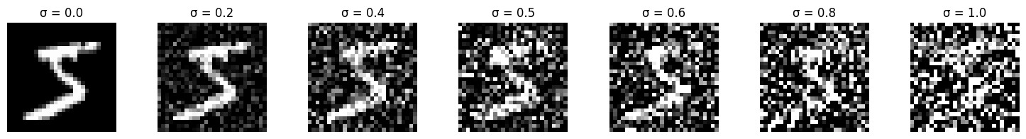
Given a clean image x₁, we generate noisy training pairs using:

$$x_t = x_0 + \sigma \cdot \epsilon, \quad \epsilon \sim \mathcal{N}(0, I)$$

where sigma controls noise level. The network learns to map noisy images back to clean ones using L2 loss.

1.2.0: Noise Visualization

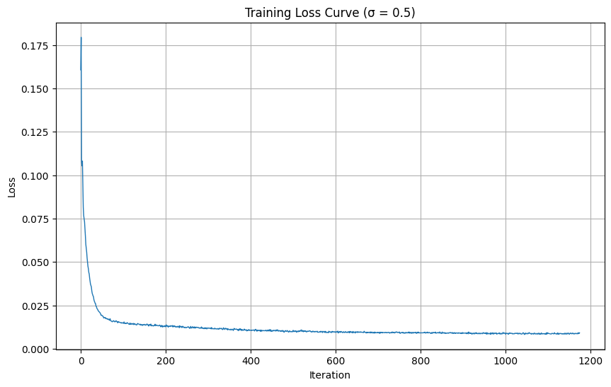
Visualization of noising process with increasing sigma values

1.2.1: Training Results

Dataset:

MNIST training set (60,000 images)

Batch Size:

256

Epochs:

Optimizer:

Adam, lr = 1e-4

Noise Level:

sigma = 0.5

Epoch 1

Epoch 5

Training loss over iterations

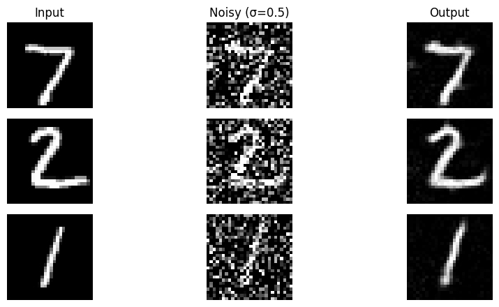
1.2.2: Out-of-Distribution Testing

The model was trained on sigma=0.5 but we evaluate on varying noise levels to test generalization:

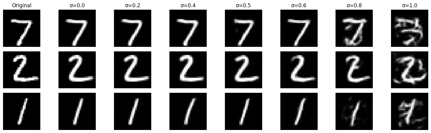
Denoising at different sigma values

Observation

The denoiser performs well near sigma=0.5 (training condition) but degrades at extreme noise levels. This demonstrates that the model learned task-specific solutions rather than generalizable denoising principles.

1.2.3: Denoising Pure Noise

We retrain the model to denoise pure Gaussian noise (x₀ = noise), effectively turning this into a generative task:

Training loss over iterations

Epoch 1

Epoch 5

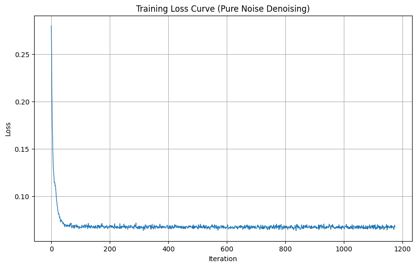
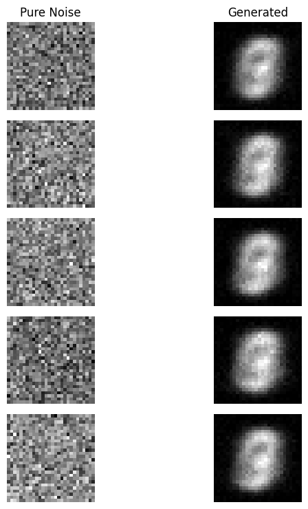
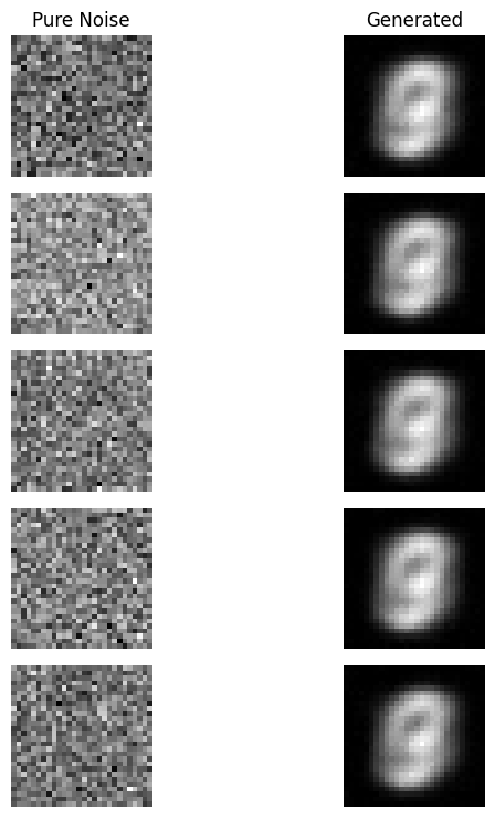
Pure Noise Denoising Analysis

Patterns Observed: The model generates blurry digit-like shapes but lacking details.

Why This Happens: With MSE loss, the network learns to predict the centroid/mean of all training images. When trained to denoise pure noise, it averages out all digits into a single indistinct blob. This is the fundamental limitation of one-step denoising for generation.

Part 2: Flow Matching & Time-Conditioned Generation

To improve generation quality, we transition to iterative denoising using flow matching. The key insight is to learn a velocity field that continuously transforms noise into clean data.

2.1: Time Conditioning

We inject scalar timestep t into the UNet using fully-connected blocks (FCBlocks). For each FCBlock layer:

$$\text{FCBlock}: t \rightarrow [F_{\text{hidden}}] \rightarrow F_{\text{out}}$$

The embedding is applied through element-wise multiplication at key points in the network (unflatten and up1 layers), modulating the denoiser's behavior across different noise levels.

2.2: Training Time-Conditioned UNet

Dataset:

MNIST training set (shuffled)

Batch Size:

Hidden Dimension:

D = 64

Optimizer:

Adam, lr = 1e-2

LR Scheduler:

ExponentialLR, $ \gamma = 0.1^{\frac{1.0}{\text{num epochs}}} $

Time-conditioned UNet training loss curve

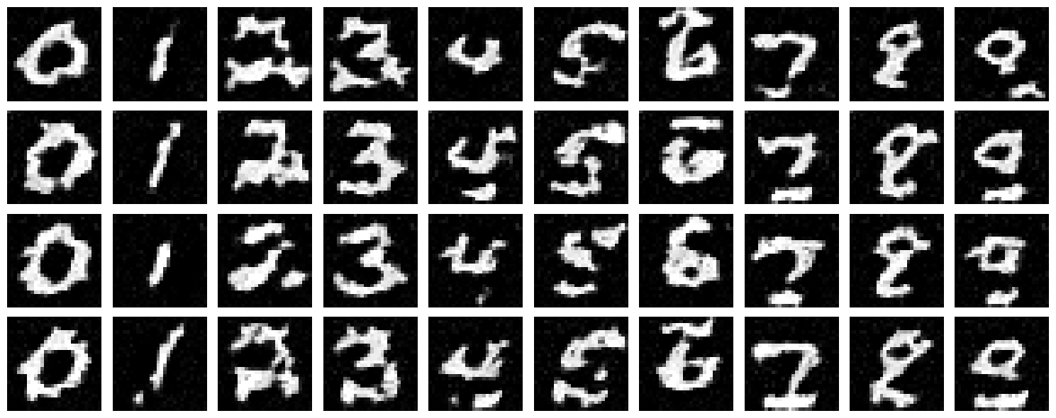
2.3: Sampling & Generation Results

Using the trained model, we iteratively denoise pure noise to generate MNIST digits. Sample quality improves significantly over training epochs:

Epoch 1

Epoch 5

Epoch 10

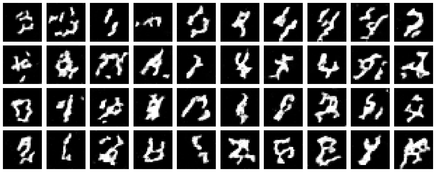
Generation Quality

While results show clear digit structures, they lack fine details compared to training data. This is expected given the simplified model and limited training time. Iterative denoising is fundamentally more powerful than one-step approaches.

Bells & Whistles: Improving Time-Conditioned UNet

The basic time-conditioned model produces reasonable but imperfect results. We implement several improvements:

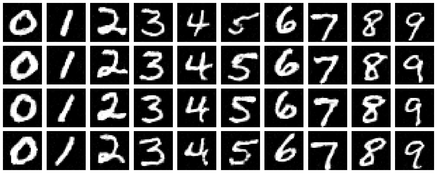
Improvement 1: Extended Training Schedule

Approach: Train for 20 epochs instead of 10, allowing the network more opportunities to refine weights.

Result: Smoother generation with better digit structure and reduced artifacts.

Improvement 2: Increased Sampling Steps

Approach: Increase sampling timesteps from 50 to 100 for finer iterative refinement during generation.

Result: Higher quality generated images with smoother transitions between noise levels.

Original (10 epochs, 50 steps)

Improved (20 epochs, 100 steps)

Improvement Summary

Best Result: Combining extended training (20 epochs) + increased sampling steps (100 timesteps) produces visibly cleaner, more coherent digit generation. More training time and finer-grained denoising steps lead to significantly improved generation quality.

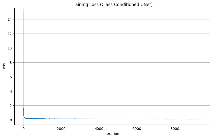
2.4-2.5: Class-Conditioned UNet

We add class conditioning via one-hot vectors with 10% dropout for unconditional guidance capability:

Class Conditioning:

One-hot vectors [0-9], 10% dropout

Additional FCBlocks:

2 (fc1_c, fc2_c for class embedding)

Training Epochs:

10 (faster convergence with guidance)

Class-conditioned UNet training loss

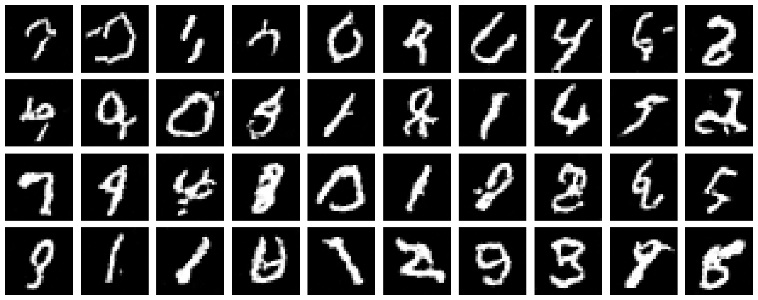
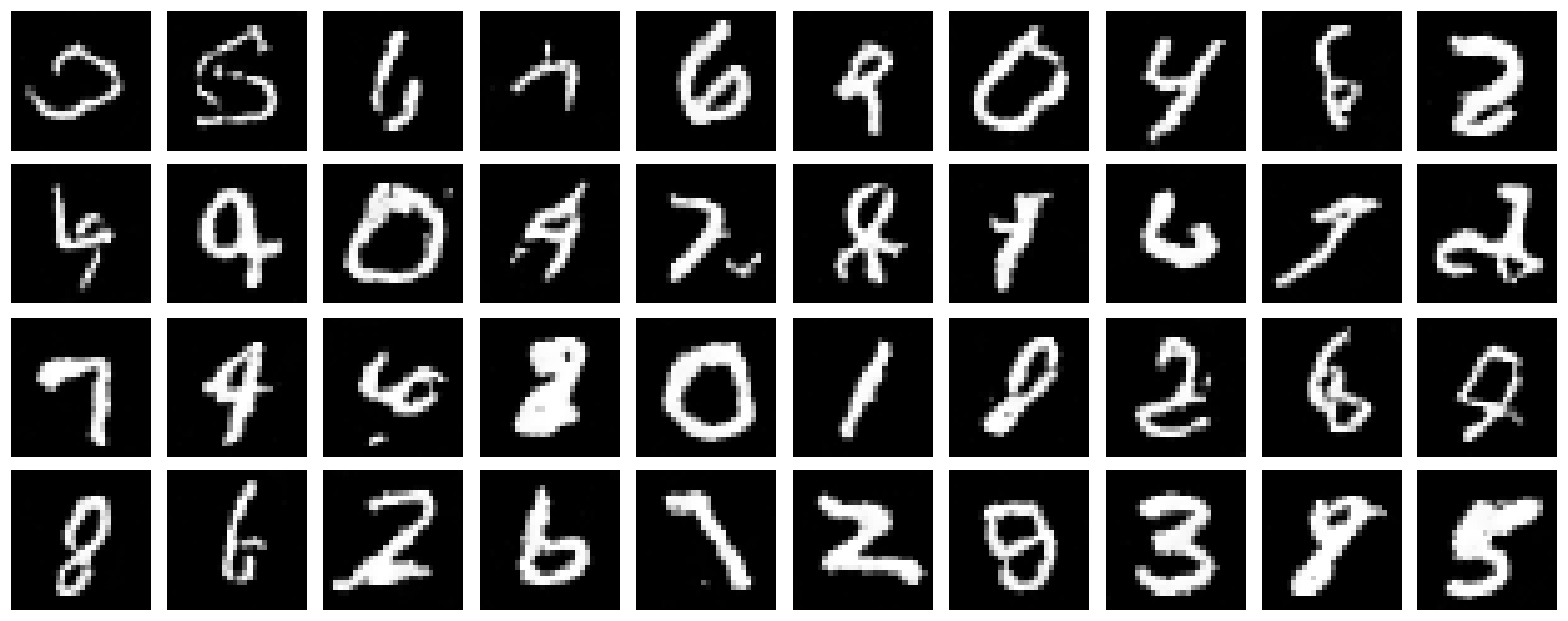
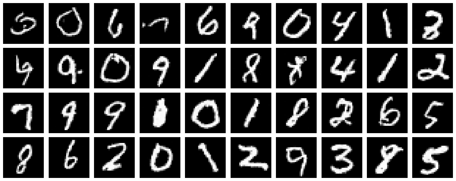
2.6: Sampling with Class Guidance

Using classifier-free guidance with scale γ = 5, we generate 4 instances of each digit 0-9:

Epoch 1

Epoch 5

Epoch 10

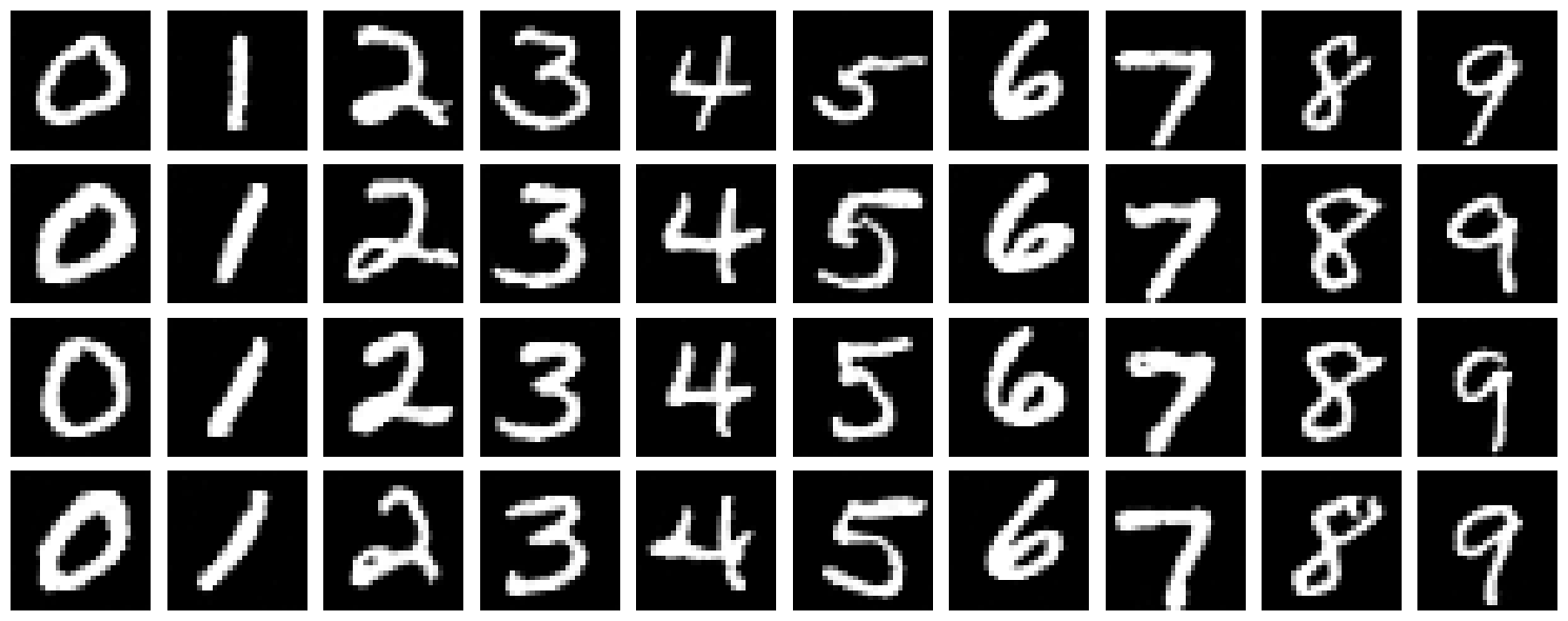
Class-Guided Generation

Class conditioning dramatically improves generation quality. The model learns to generate digits that are clearly recognizable by their class, with consistent style within each digit type. Guidance helps enforce semantic consistency.

Removing the Learning Rate Scheduler

We investigate whether the exponential LR scheduler is necessary for good performance:

Approach: Fixed Learning Rate Tuning

Strategy: Replace exponential decay with a fixed, higher learning rate. We found that $\text{lr} = 2 \times 10^{-2}$ with 20 epochs achieves comparable convergence without scheduler overhead.

Finding: A constant learning rate of $2 \times 10^{-2}$ maintains competitive performance without exponential decay complexity.

Benefit: Simpler training code and fewer hyperparameters.

With LR Scheduler (Original)

Fixed LR = $2 \times 10^{-2}$ (No Scheduler)

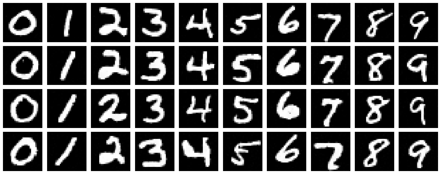
Scheduler Removal Summary

A constant learning rate of $2 \times 10^{-2}$ trained for 20 epochs achieves comparable final performance without exponential decay. Properly tuned fixed rates work exceptionally well for MNIST flow matching.

Conclusion

🎯 Key Learnings

One-step denoising averages out to mode-seeking behavior (centroid)
Iterative denoising with flow matching enables high-quality generation
Time conditioning allows single network to handle all noise levels
Class conditioning + guidance improves semantic control
Architecture design and training duration significantly impact results

🔧 Technical Takeaways

UNet with skip connections preserve spatial information
FCBlocks enable modulation across timestep/class dimensions
Classifier-free guidance (10% unconditional dropout) is essential
Sinusoidal embeddings > linear embeddings for temporal signals
Proper learning rate tuning can replace scheduler complexity